16 dplyr

- Link: https://dplyr.tidyverse.org/
- Index of Functions: https://dplyr.tidyverse.org/reference/index.html
- Cheat Sheet: https://github.com/rstudio/cheatsheets/blob/master/data-transformation.pdf
- Chapter of R for Data Science: https://r4ds.had.co.nz/transform.html
- Unofficial Example: https://rpubs.com/williamsurles/293454
suppressPackageStartupMessages(
  library(dplyr)
)
16.0.1 Example Data
Import the example data. This data represents benthic macroinvertebrate data collected in the littoral zone of Onondaga, Otisco, and Cazenovia lakes
taxa.df <- file.path("data",
                     "zms_thesis-macro_2017-06-18.csv") %>%
  read.csv(stringsAsFactors = FALSE)

DT::datatable(taxa.df, options = list(scrollX = TRUE))
env.df <- file.path("data",
"zms_thesis-env_2017-06-18.csv") %>%
read.csv(stringsAsFactors = FALSE)
DT::datatable(env.df, options = list(scrollX = TRUE))16.0.2 Rename
- Definition: give a new name to a specified column(s).
- Link: https://dplyr.tidyverse.org/reference/select.html
In the example below, the columns lat and long are renamed to latitude and longitude, respectively. If names(taxa.df) is called, elements 5 and 6 are now represented by “latitude” and “longitude”, respectively.
taxa.df <- taxa.df %>%
  rename(latitude = lat,
         longitude = long)

names(taxa.df)
## [1] "unique_id" "lake" "station_id" "sample_number"
## [5] "latitude" "longitude" "agency_code" "method"
## [9] "date" "count" "life_stage" "final_id"
## [13] "taxon_level" "phylum" "subphylum" "class"
## [17] "subclass" "order" "suborder" "family"
## [21] "subfamily" "tribe" "genus" "species"
## [25] "picked" "squares"16.0.3 Filter
- Definition: subset rows using logical statements.
- Link: https://dplyr.tidyverse.org/reference/filter.html
In the example below, taxa.df is subset to only include rows where the unique_id column matches the string “caz_1_1”.
filter.df <- taxa.df %>%
  filter(unique_id == "caz_1_1")

DT::datatable(filter.df, options = list(scrollX = TRUE))
You can apply multiple filters separate by commas. The filters are applied from the top down. In the example below, two filters are applied within the filter() call:
unique_id == "caz_1_1"order %in% c("ephemeroptera", "trichoptera")
The first logical statement is the same as the filter from the code chunk above, which keeps only rows associated with the sample “caz_1_1”. Then, the order column is subset the data to only include rows represented by ephemeroptera (mayfly) or trichoptera (caddisfly) taxa.
filter.df <- taxa.df %>%
  filter(unique_id == "caz_1_1",
         order %in% c("ephemeroptera", "trichoptera"))

DT::datatable(filter.df, options = list(scrollX = TRUE))
16.0.4 Select
- Definition: subset of columns.
- Link: https://dplyr.tidyverse.org/reference/select.html
Often we are not interested in all columns in a data frame. select() can be used to subset the columns to only include columns of interest. In the example below, the filter.df data frame, created in the Filter section, is subset to only include three columns: 1) final_id, count, and unique_id.
select.df <- filter.df %>%
  select(unique_id, final_id, count)

knitr::kable(select.df)| unique_id | final_id | count |
|---|---|---|
| caz_1_1 | baetidae | 1 |
| caz_1_1 | caenis | 14 |
| caz_1_1 | agraylea | 1 |
| caz_1_1 | oxyethira | 2 |
| caz_1_1 | hydroptilidae | 1 |
The same operation can be performed by chaining the functions together with the pipe operator. taxa.df is first filtered to only include rows that meet our specified logical statements and then only the columns unique_id, final_id, and count are retained.
select.df <- taxa.df %>%
  filter(unique_id == "caz_1_1",
         order %in% c("ephemeroptera", "trichoptera")) %>%
  select(unique_id, final_id, count)

knitr::kable(select.df)| unique_id | final_id | count |
|---|---|---|
| caz_1_1 | baetidae | 1 |
| caz_1_1 | caenis | 14 |
| caz_1_1 | agraylea | 1 |
| caz_1_1 | oxyethira | 2 |
| caz_1_1 | hydroptilidae | 1 |
Reorder columns. Maybe you would prefer to see the columns in the following order:
final_idunique_idcount
reorder.df <- taxa.df %>%
  filter(unique_id == "caz_1_1",
         order %in% c("ephemeroptera", "trichoptera")) %>%
  select(final_id, unique_id, count)

knitr::kable(reorder.df)| final_id | unique_id | count |
|---|---|---|
| baetidae | caz_1_1 | 1 |
| caenis | caz_1_1 | 14 |
| agraylea | caz_1_1 | 1 |
| oxyethira | caz_1_1 | 2 |
| hydroptilidae | caz_1_1 | 1 |
16.0.4.1 everything
- Definition: helper function for
select. Specifies all columns not already specified in theselect()call. - Link:
For example, maybe we want to see the first three columns reordered but the remaining columns to remain in the same order. Without everything(), we would need to specify each column in the select() call. With everything(), we can specify the first three columns to be lake, station_id, and sample_number followed by everything(). The columns will then be reordered accordingly (lake, station_id, sample_number, unique_id, etc.).
reorder.df <- taxa.df %>%
  filter(unique_id == "caz_1_1",
         order %in% c("ephemeroptera", "trichoptera")) %>%
  select(lake, station_id, sample_number, everything())

DT::datatable(reorder.df, options = list(scrollX = TRUE))
16.0.5 distinct
- Definition: remove duplicate rows.
- Link: https://dplyr.tidyverse.org/reference/distinct.html
After performing a subsetting columns with select(), it may be beneficial to subsequently run distinct() to remove any duplicate rows.
Maybe we are just interested in viewing basic sample information such as lake, station_id, and sample_number. If select() is performed to subset the data frame to only represent these columns, then there will be many duplicate rows. The reason for this is in the original taxa.df data frame there are multiple taxa observed per sample. lake, station_id, and sample_number are associated accordingly with the taxa, and therefore lake, station_id, and sample_number are represented many times.
nondistinct.df <- taxa.df %>%
  select(lake, station_id, sample_number)

DT::datatable(nondistinct.df,
              options = list(columnDefs = list(list(className = 'dt-center', targets = 0:3))))
distinct() will remove the duplicate rows present in the output above. This is a very simple call, which requires no input.
distinct.df <- taxa.df %>%
  select(lake, station_id, sample_number) %>%
  distinct()

DT::datatable(distinct.df,
              options = list(columnDefs = list(list(className = 'dt-center', targets = 0:3))))
16.0.6 mutate
- Definition: create or overwrite columns.
- Link: https://dplyr.tidyverse.org/reference/mutate.html
In the example below, I use the select() and distinct() combination from the distinct section and then filter the data frame to only include rows where lake equals “caz”. The distinct() call has insured that each row is unique but there is not a single column that could be used to uniquely identify a given sample. Using mutate() we can create a new column, called new_id, that concatenates the station_id and sample_number columns into a single value separated by an underscore (paste(station_id, sample_number, sep = "_")).
mutate.df <- taxa.df %>%
  select(lake, station_id, sample_number) %>%
  distinct() %>%
  filter(lake == "caz") %>%
  mutate(new_id = paste(station_id, sample_number,
                        sep = "_"))

DT::datatable(mutate.df,
              options = list(columnDefs = list(list(className = 'dt-center', targets = 0:4))))
Maybe a second type of unique identifier is wanted for certain subsequent processes. mutate() allows for the creation of one or more columns within a single call. In the example below, new_id is created as it was in the example above but is followed by the creation of date_id. date_id is created by concatenating new_id and date columns. Therefore, a single mutate() call has created two new columns. Additionally, we can see that columns created downstream (date_id) can reference columns created upstream (new_id) within the mutate() call.
mutate.df <- taxa.df %>%
  select(lake, station_id, sample_number, date) %>%
  distinct() %>%
  filter(lake == "caz") %>%
  mutate(new_id = paste(station_id, sample_number,
                        sep = "_"),
         date_id = paste(new_id, date,
                         sep = "_"))

DT::datatable(mutate.df,
              options = list(columnDefs = list(list(className = 'dt-center', targets = 0:6))))
16.0.7 group_by
- Definition: aggregate by specified columns.
- Link: https://dplyr.tidyverse.org/reference/group_by.html
Calling group_by() will aggregate the data by the column(s) specified but alone will not alter the content of the data frame.
group.df <- taxa.df %>%
  filter(unique_id %in% c("caz_1_1", "caz_1_2")) %>%
  select(unique_id, final_id, count) %>%
  group_by(unique_id)

knitr::kable(group.df)| unique_id | final_id | count |
|---|---|---|
| caz_1_1 | physa | 1 |
| caz_1_1 | gyraulus | 1 |
| caz_1_1 | bezzia | 5 |
| caz_1_1 | mallochohelea | 7 |
| caz_1_1 | chironomus | 1 |
| caz_1_1 | dicrotendipes | 3 |
| caz_1_1 | paratanytarsus | 34 |
| caz_1_1 | cricotopus | 1 |
| caz_1_1 | psectrocladius | 5 |
| caz_1_1 | thienemanniella | 4 |
| caz_1_1 | krenopelopia | 9 |
| caz_1_1 | procladius | 1 |
| caz_1_1 | hemerodromia | 1 |
| caz_1_1 | baetidae | 1 |
| caz_1_1 | caenis | 14 |
| caz_1_1 | acentria | 1 |
| caz_1_1 | enallagma | 1 |
| caz_1_1 | agraylea | 1 |
| caz_1_1 | oxyethira | 2 |
| caz_1_1 | hydroptilidae | 1 |
| caz_1_1 | gammarus | 2 |
| caz_1_1 | hyalella | 14 |
| caz_1_1 | caecidotea | 2 |
| caz_1_2 | amnicola_grana | 2 |
| caz_1_2 | physa | 27 |
| caz_1_2 | gyraulus_parvus | 1 |
| caz_1_2 | helisoma_anceps | 2 |
| caz_1_2 | promenetus_exacuous | 5 |
| caz_1_2 | valvata | 1 |
| caz_1_2 | bezzia | 9 |
| caz_1_2 | mallochohelea | 2 |
| caz_1_2 | chironomus | 5 |
| caz_1_2 | dicrotendipes | 4 |
| caz_1_2 | microtendipes | 1 |
| caz_1_2 | polypedilum | 2 |
| caz_1_2 | pseudochironomus | 1 |
| caz_1_2 | rheotanytarsus | 2 |
| caz_1_2 | thienemanniella | 1 |
| caz_1_2 | ablabesmyia | 5 |
| caz_1_2 | callibaetis | 1 |
| caz_1_2 | caenis | 1 |
| caz_1_2 | caenidae | 2 |
| caz_1_2 | acentria | 1 |
| caz_1_2 | mystacides | 2 |
| caz_1_2 | gammarus | 1 |
| caz_1_2 | hyalella | 13 |
| caz_1_2 | caecidotea | 9 |
The image below shows “under the hood”" information about group.df from the Environment Tab before and after the group_by() call is made. We do not need to focus on the details associated with this “under the hood” information but this way we can view the change made by the group_by() call; unlike the table shown above, which does not provided any indication that the data has been aggregated.

We can follow group_by() by a mutate() call to calculate a single value per group. Each group variable is replicated for each row within a group. In the example below, we are aggregating by two unique_ids (group_by(unique_id); “caz_1_1” and “caz_1_2”) and finding the total number of organisms identified within each group (mutate(total = sum(count))). The sum() function returns one number per group. mutate() then replicates this one number for all rows within a group.
group.df <- taxa.df %>%
  filter(unique_id %in% c("caz_1_1", "caz_1_2")) %>%
  select(unique_id, final_id, count) %>%
  group_by(unique_id) %>%
  mutate(total = sum(count))

knitr::kable(group.df)| unique_id | final_id | count | total |
|---|---|---|---|
| caz_1_1 | physa | 1 | 112 |
| caz_1_1 | gyraulus | 1 | 112 |
| caz_1_1 | bezzia | 5 | 112 |
| caz_1_1 | mallochohelea | 7 | 112 |
| caz_1_1 | chironomus | 1 | 112 |
| caz_1_1 | dicrotendipes | 3 | 112 |
| caz_1_1 | paratanytarsus | 34 | 112 |
| caz_1_1 | cricotopus | 1 | 112 |
| caz_1_1 | psectrocladius | 5 | 112 |
| caz_1_1 | thienemanniella | 4 | 112 |
| caz_1_1 | krenopelopia | 9 | 112 |
| caz_1_1 | procladius | 1 | 112 |
| caz_1_1 | hemerodromia | 1 | 112 |
| caz_1_1 | baetidae | 1 | 112 |
| caz_1_1 | caenis | 14 | 112 |
| caz_1_1 | acentria | 1 | 112 |
| caz_1_1 | enallagma | 1 | 112 |
| caz_1_1 | agraylea | 1 | 112 |
| caz_1_1 | oxyethira | 2 | 112 |
| caz_1_1 | hydroptilidae | 1 | 112 |
| caz_1_1 | gammarus | 2 | 112 |
| caz_1_1 | hyalella | 14 | 112 |
| caz_1_1 | caecidotea | 2 | 112 |
| caz_1_2 | amnicola_grana | 2 | 100 |
| caz_1_2 | physa | 27 | 100 |
| caz_1_2 | gyraulus_parvus | 1 | 100 |
| caz_1_2 | helisoma_anceps | 2 | 100 |
| caz_1_2 | promenetus_exacuous | 5 | 100 |
| caz_1_2 | valvata | 1 | 100 |
| caz_1_2 | bezzia | 9 | 100 |
| caz_1_2 | mallochohelea | 2 | 100 |
| caz_1_2 | chironomus | 5 | 100 |
| caz_1_2 | dicrotendipes | 4 | 100 |
| caz_1_2 | microtendipes | 1 | 100 |
| caz_1_2 | polypedilum | 2 | 100 |
| caz_1_2 | pseudochironomus | 1 | 100 |
| caz_1_2 | rheotanytarsus | 2 | 100 |
| caz_1_2 | thienemanniella | 1 | 100 |
| caz_1_2 | ablabesmyia | 5 | 100 |
| caz_1_2 | callibaetis | 1 | 100 |
| caz_1_2 | caenis | 1 | 100 |
| caz_1_2 | caenidae | 2 | 100 |
| caz_1_2 | acentria | 1 | 100 |
| caz_1_2 | mystacides | 2 | 100 |
| caz_1_2 | gammarus | 1 | 100 |
| caz_1_2 | hyalella | 13 | 100 |
| caz_1_2 | caecidotea | 9 | 100 |
This example can be taken one step further to calculate relative abundance (i.e., the percentage of the sample represented by each taxon) by adding percent = count / total * 100 to the mutate() call.
group.df <- taxa.df %>%
  filter(unique_id %in% c("caz_1_1", "caz_1_2")) %>%
  select(unique_id, final_id, count) %>%
  group_by(unique_id) %>%
  mutate(total = sum(count),
         percent = count / total * 100)

knitr::kable(group.df)| unique_id | final_id | count | total | percent |
|---|---|---|---|---|
| caz_1_1 | physa | 1 | 112 | 0.8928571 |
| caz_1_1 | gyraulus | 1 | 112 | 0.8928571 |
| caz_1_1 | bezzia | 5 | 112 | 4.4642857 |
| caz_1_1 | mallochohelea | 7 | 112 | 6.2500000 |
| caz_1_1 | chironomus | 1 | 112 | 0.8928571 |
| caz_1_1 | dicrotendipes | 3 | 112 | 2.6785714 |
| caz_1_1 | paratanytarsus | 34 | 112 | 30.3571429 |
| caz_1_1 | cricotopus | 1 | 112 | 0.8928571 |
| caz_1_1 | psectrocladius | 5 | 112 | 4.4642857 |
| caz_1_1 | thienemanniella | 4 | 112 | 3.5714286 |
| caz_1_1 | krenopelopia | 9 | 112 | 8.0357143 |
| caz_1_1 | procladius | 1 | 112 | 0.8928571 |
| caz_1_1 | hemerodromia | 1 | 112 | 0.8928571 |
| caz_1_1 | baetidae | 1 | 112 | 0.8928571 |
| caz_1_1 | caenis | 14 | 112 | 12.5000000 |
| caz_1_1 | acentria | 1 | 112 | 0.8928571 |
| caz_1_1 | enallagma | 1 | 112 | 0.8928571 |
| caz_1_1 | agraylea | 1 | 112 | 0.8928571 |
| caz_1_1 | oxyethira | 2 | 112 | 1.7857143 |
| caz_1_1 | hydroptilidae | 1 | 112 | 0.8928571 |
| caz_1_1 | gammarus | 2 | 112 | 1.7857143 |
| caz_1_1 | hyalella | 14 | 112 | 12.5000000 |
| caz_1_1 | caecidotea | 2 | 112 | 1.7857143 |
| caz_1_2 | amnicola_grana | 2 | 100 | 2.0000000 |
| caz_1_2 | physa | 27 | 100 | 27.0000000 |
| caz_1_2 | gyraulus_parvus | 1 | 100 | 1.0000000 |
| caz_1_2 | helisoma_anceps | 2 | 100 | 2.0000000 |
| caz_1_2 | promenetus_exacuous | 5 | 100 | 5.0000000 |
| caz_1_2 | valvata | 1 | 100 | 1.0000000 |
| caz_1_2 | bezzia | 9 | 100 | 9.0000000 |
| caz_1_2 | mallochohelea | 2 | 100 | 2.0000000 |
| caz_1_2 | chironomus | 5 | 100 | 5.0000000 |
| caz_1_2 | dicrotendipes | 4 | 100 | 4.0000000 |
| caz_1_2 | microtendipes | 1 | 100 | 1.0000000 |
| caz_1_2 | polypedilum | 2 | 100 | 2.0000000 |
| caz_1_2 | pseudochironomus | 1 | 100 | 1.0000000 |
| caz_1_2 | rheotanytarsus | 2 | 100 | 2.0000000 |
| caz_1_2 | thienemanniella | 1 | 100 | 1.0000000 |
| caz_1_2 | ablabesmyia | 5 | 100 | 5.0000000 |
| caz_1_2 | callibaetis | 1 | 100 | 1.0000000 |
| caz_1_2 | caenis | 1 | 100 | 1.0000000 |
| caz_1_2 | caenidae | 2 | 100 | 2.0000000 |
| caz_1_2 | acentria | 1 | 100 | 1.0000000 |
| caz_1_2 | mystacides | 2 | 100 | 2.0000000 |
| caz_1_2 | gammarus | 1 | 100 | 1.0000000 |
| caz_1_2 | hyalella | 13 | 100 | 13.0000000 |
| caz_1_2 | caecidotea | 9 | 100 | 9.0000000 |
16.0.7.1 ungroup
- Definition: remove the aggregation applied by
group_by(). - Link: https://dplyr.tidyverse.org/reference/group_by.html
Once the calculations that required aggregation (i.e., group_by()) are complete, make sure to remove the aggregation from the data frame using ungroup(). If you forget to do this, R will continue to try to apply the aggregation to future calculations, which will most likely be inappropriate. Generally, you will eventually get an error message if you forget to use ungroup().
ungroup.df <- taxa.df %>%
  filter(unique_id %in% c("caz_1_1", "caz_1_2")) %>%
  select(unique_id, final_id, count) %>%
  group_by(unique_id) %>%
  mutate(total = sum(count),
         percent = count / total * 100) %>%
  ungroup()

knitr::kable(ungroup.df)| unique_id | final_id | count | total | percent |
|---|---|---|---|---|
| caz_1_1 | physa | 1 | 112 | 0.8928571 |
| caz_1_1 | gyraulus | 1 | 112 | 0.8928571 |
| caz_1_1 | bezzia | 5 | 112 | 4.4642857 |
| caz_1_1 | mallochohelea | 7 | 112 | 6.2500000 |
| caz_1_1 | chironomus | 1 | 112 | 0.8928571 |
| caz_1_1 | dicrotendipes | 3 | 112 | 2.6785714 |
| caz_1_1 | paratanytarsus | 34 | 112 | 30.3571429 |
| caz_1_1 | cricotopus | 1 | 112 | 0.8928571 |
| caz_1_1 | psectrocladius | 5 | 112 | 4.4642857 |
| caz_1_1 | thienemanniella | 4 | 112 | 3.5714286 |
| caz_1_1 | krenopelopia | 9 | 112 | 8.0357143 |
| caz_1_1 | procladius | 1 | 112 | 0.8928571 |
| caz_1_1 | hemerodromia | 1 | 112 | 0.8928571 |
| caz_1_1 | baetidae | 1 | 112 | 0.8928571 |
| caz_1_1 | caenis | 14 | 112 | 12.5000000 |
| caz_1_1 | acentria | 1 | 112 | 0.8928571 |
| caz_1_1 | enallagma | 1 | 112 | 0.8928571 |
| caz_1_1 | agraylea | 1 | 112 | 0.8928571 |
| caz_1_1 | oxyethira | 2 | 112 | 1.7857143 |
| caz_1_1 | hydroptilidae | 1 | 112 | 0.8928571 |
| caz_1_1 | gammarus | 2 | 112 | 1.7857143 |
| caz_1_1 | hyalella | 14 | 112 | 12.5000000 |
| caz_1_1 | caecidotea | 2 | 112 | 1.7857143 |
| caz_1_2 | amnicola_grana | 2 | 100 | 2.0000000 |
| caz_1_2 | physa | 27 | 100 | 27.0000000 |
| caz_1_2 | gyraulus_parvus | 1 | 100 | 1.0000000 |
| caz_1_2 | helisoma_anceps | 2 | 100 | 2.0000000 |
| caz_1_2 | promenetus_exacuous | 5 | 100 | 5.0000000 |
| caz_1_2 | valvata | 1 | 100 | 1.0000000 |
| caz_1_2 | bezzia | 9 | 100 | 9.0000000 |
| caz_1_2 | mallochohelea | 2 | 100 | 2.0000000 |
| caz_1_2 | chironomus | 5 | 100 | 5.0000000 |
| caz_1_2 | dicrotendipes | 4 | 100 | 4.0000000 |
| caz_1_2 | microtendipes | 1 | 100 | 1.0000000 |
| caz_1_2 | polypedilum | 2 | 100 | 2.0000000 |
| caz_1_2 | pseudochironomus | 1 | 100 | 1.0000000 |
| caz_1_2 | rheotanytarsus | 2 | 100 | 2.0000000 |
| caz_1_2 | thienemanniella | 1 | 100 | 1.0000000 |
| caz_1_2 | ablabesmyia | 5 | 100 | 5.0000000 |
| caz_1_2 | callibaetis | 1 | 100 | 1.0000000 |
| caz_1_2 | caenis | 1 | 100 | 1.0000000 |
| caz_1_2 | caenidae | 2 | 100 | 2.0000000 |
| caz_1_2 | acentria | 1 | 100 | 1.0000000 |
| caz_1_2 | mystacides | 2 | 100 | 2.0000000 |
| caz_1_2 | gammarus | 1 | 100 | 1.0000000 |
| caz_1_2 | hyalella | 13 | 100 | 13.0000000 |
| caz_1_2 | caecidotea | 9 | 100 | 9.0000000 |
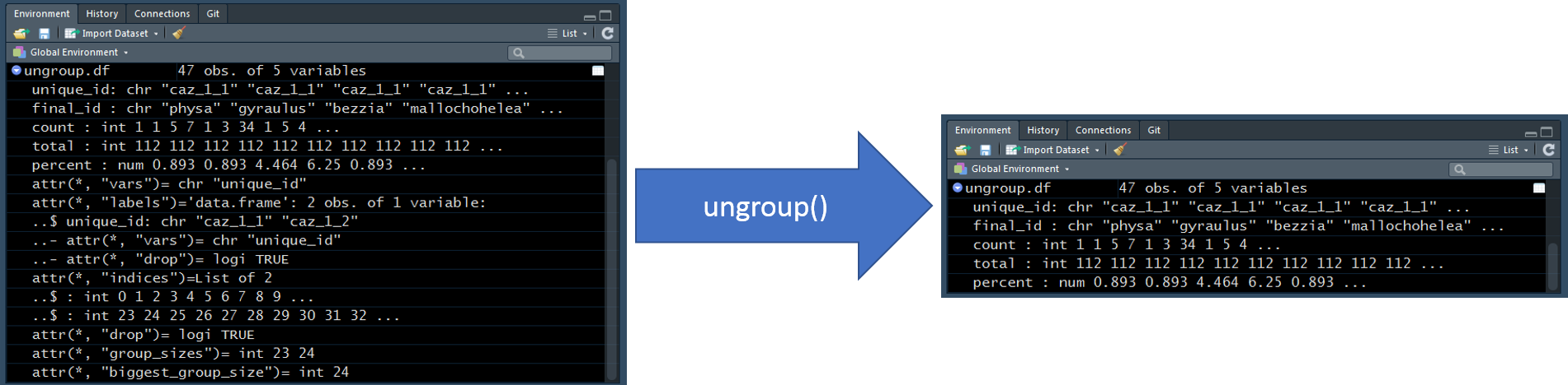
The image below shows “under the hood”" information about ungroup.df from the Environment Tab before and after the ungroup() call is made. We do not need to focus on the details associated with this “under the hood” information but this way we can view the change made by the ungroup() call; unlike the table shown above, which does not provided any indication that the data has been unaggregated.
16.0.8 summarize
- Definition: creates or overwrites columns but only retains columns specified in
group_by()and the column(s) created in thesummarize()call. This function requiresgroup_by()to be called in advance. - Link: https://dplyr.tidyverse.org/reference/summarise.html
In the group_by example, we calculated the percentage of the sample comprised by each final_id taxon. final_id represents the highest taxonomic resolution for which these taxa were identified; therefore, each row represented a unique taxon.
What if we want to explore these samples at a lower resolution? In the example below, the taxa are represented at the order-level. The percent calculations are correct but, in many cases, the same taxon is represented more than once. This is a poor representation of the data. summarize() can help us solve this issue in the subsequent code chunks.
sub.df <- taxa.df %>%
  filter(unique_id %in% c("caz_1_1", "caz_1_2")) %>%
  select(unique_id, order, count) %>%
  group_by(unique_id)  %>%
  mutate(total = sum(count),
         percent = count / total * 100) %>%
  ungroup()

knitr::kable(sub.df)| unique_id | order | count | total | percent |
|---|---|---|---|---|
| caz_1_1 | basommatophora | 1 | 112 | 0.8928571 |
| caz_1_1 | basommatophora | 1 | 112 | 0.8928571 |
| caz_1_1 | diptera | 5 | 112 | 4.4642857 |
| caz_1_1 | diptera | 7 | 112 | 6.2500000 |
| caz_1_1 | diptera | 1 | 112 | 0.8928571 |
| caz_1_1 | diptera | 3 | 112 | 2.6785714 |
| caz_1_1 | diptera | 34 | 112 | 30.3571429 |
| caz_1_1 | diptera | 1 | 112 | 0.8928571 |
| caz_1_1 | diptera | 5 | 112 | 4.4642857 |
| caz_1_1 | diptera | 4 | 112 | 3.5714286 |
| caz_1_1 | diptera | 9 | 112 | 8.0357143 |
| caz_1_1 | diptera | 1 | 112 | 0.8928571 |
| caz_1_1 | diptera | 1 | 112 | 0.8928571 |
| caz_1_1 | ephemeroptera | 1 | 112 | 0.8928571 |
| caz_1_1 | ephemeroptera | 14 | 112 | 12.5000000 |
| caz_1_1 | lepidoptera | 1 | 112 | 0.8928571 |
| caz_1_1 | odonata | 1 | 112 | 0.8928571 |
| caz_1_1 | trichoptera | 1 | 112 | 0.8928571 |
| caz_1_1 | trichoptera | 2 | 112 | 1.7857143 |
| caz_1_1 | trichoptera | 1 | 112 | 0.8928571 |
| caz_1_1 | amphipoda | 2 | 112 | 1.7857143 |
| caz_1_1 | amphipoda | 14 | 112 | 12.5000000 |
| caz_1_1 | isopoda | 2 | 112 | 1.7857143 |
| caz_1_2 | neotaenioglossa | 2 | 100 | 2.0000000 |
| caz_1_2 | basommatophora | 27 | 100 | 27.0000000 |
| caz_1_2 | basommatophora | 1 | 100 | 1.0000000 |
| caz_1_2 | basommatophora | 2 | 100 | 2.0000000 |
| caz_1_2 | basommatophora | 5 | 100 | 5.0000000 |
| caz_1_2 | heterostropha | 1 | 100 | 1.0000000 |
| caz_1_2 | diptera | 9 | 100 | 9.0000000 |
| caz_1_2 | diptera | 2 | 100 | 2.0000000 |
| caz_1_2 | diptera | 5 | 100 | 5.0000000 |
| caz_1_2 | diptera | 4 | 100 | 4.0000000 |
| caz_1_2 | diptera | 1 | 100 | 1.0000000 |
| caz_1_2 | diptera | 2 | 100 | 2.0000000 |
| caz_1_2 | diptera | 1 | 100 | 1.0000000 |
| caz_1_2 | diptera | 2 | 100 | 2.0000000 |
| caz_1_2 | diptera | 1 | 100 | 1.0000000 |
| caz_1_2 | diptera | 5 | 100 | 5.0000000 |
| caz_1_2 | ephemeroptera | 1 | 100 | 1.0000000 |
| caz_1_2 | ephemeroptera | 1 | 100 | 1.0000000 |
| caz_1_2 | ephemeroptera | 2 | 100 | 2.0000000 |
| caz_1_2 | lepidoptera | 1 | 100 | 1.0000000 |
| caz_1_2 | trichoptera | 2 | 100 | 2.0000000 |
| caz_1_2 | amphipoda | 1 | 100 | 1.0000000 |
| caz_1_2 | amphipoda | 13 | 100 | 13.0000000 |
| caz_1_2 | isopoda | 9 | 100 | 9.0000000 |
The most intuitive way to solve this problem, to sum the counts by unique and order columns before calculating the percentages, which can be down with a combination of group_by() and summarize().
- Apply
group_by()to theunique_idandordercolumns.group_by(unique_id, order)
- Use
summarize()in the same waymutate()was applied in the mutate section. In this case, thecountwill be overwritten by the sum of the counts aggregated by theunique_idandordercolumns.summarize(count = sum(count))
- Use
ungroup()to remove the groupings created withgroup_by().
In the table output, we can see that each taxon, order, is only represented once per sample, unique_id.
summarize.df <- taxa.df %>%
  filter(unique_id %in% c("caz_1_1", "caz_1_2")) %>%
  select(unique_id, order, count) %>%
  group_by(unique_id, order) %>%
  summarize(count = sum(count)) %>%
  ungroup()

knitr::kable(summarize.df)| unique_id | order | count |
|---|---|---|
| caz_1_1 | amphipoda | 16 |
| caz_1_1 | basommatophora | 2 |
| caz_1_1 | diptera | 71 |
| caz_1_1 | ephemeroptera | 15 |
| caz_1_1 | isopoda | 2 |
| caz_1_1 | lepidoptera | 1 |
| caz_1_1 | odonata | 1 |
| caz_1_1 | trichoptera | 4 |
| caz_1_2 | amphipoda | 14 |
| caz_1_2 | basommatophora | 35 |
| caz_1_2 | diptera | 32 |
| caz_1_2 | ephemeroptera | 4 |
| caz_1_2 | heterostropha | 1 |
| caz_1_2 | isopoda | 9 |
| caz_1_2 | lepidoptera | 1 |
| caz_1_2 | neotaenioglossa | 2 |
| caz_1_2 | trichoptera | 2 |
To calculate the percentage of each order, apply the group_by(), mutate(), and ungroup() combination from the group_by section.
summarize.df <- taxa.df %>%
  filter(unique_id %in% c("caz_1_1", "caz_1_2")) %>%
  select(unique_id, order, count) %>%
  group_by(unique_id, order) %>%
  summarize(count = sum(count)) %>%
  ungroup() %>%
  group_by(unique_id) %>%
  mutate(total = sum(count),
         percent = count / total * 100) %>%
  ungroup()

knitr::kable(summarize.df)| unique_id | order | count | total | percent |
|---|---|---|---|---|
| caz_1_1 | amphipoda | 16 | 112 | 14.2857143 |
| caz_1_1 | basommatophora | 2 | 112 | 1.7857143 |
| caz_1_1 | diptera | 71 | 112 | 63.3928571 |
| caz_1_1 | ephemeroptera | 15 | 112 | 13.3928571 |
| caz_1_1 | isopoda | 2 | 112 | 1.7857143 |
| caz_1_1 | lepidoptera | 1 | 112 | 0.8928571 |
| caz_1_1 | odonata | 1 | 112 | 0.8928571 |
| caz_1_1 | trichoptera | 4 | 112 | 3.5714286 |
| caz_1_2 | amphipoda | 14 | 100 | 14.0000000 |
| caz_1_2 | basommatophora | 35 | 100 | 35.0000000 |
| caz_1_2 | diptera | 32 | 100 | 32.0000000 |
| caz_1_2 | ephemeroptera | 4 | 100 | 4.0000000 |
| caz_1_2 | heterostropha | 1 | 100 | 1.0000000 |
| caz_1_2 | isopoda | 9 | 100 | 9.0000000 |
| caz_1_2 | lepidoptera | 1 | 100 | 1.0000000 |
| caz_1_2 | neotaenioglossa | 2 | 100 | 2.0000000 |
| caz_1_2 | trichoptera | 2 | 100 | 2.0000000 |
The previous code chunk works but it is getting very long. Long code chunks make it harder for your future self or others to interpret and can make it harder to find/troubleshoot bugs. Better practice would be to break the previous code chunk into 2-3 sub-tasks.
The following code chunk into 3 sub-tasks, which should make it easier to follow process and allow us to observe the data after each sub-task is executed.
Explanation of sub-tasks below:
caz1.df: reduce the data frame down to only the rows and columns of interest. In this case, we are only interested in the two replicates from Cazenovia Lake site 1; therefore, I named the data framecaz1.dfto describe the data represented within the data frame.order.df: summarize the taxonomic counts by the sample,unique_id, and taxonomic rank,order.percent.df: calculate the percentage of each sample,unique_id, represented by each taxon,order.
caz1.df <- taxa.df %>%
  filter(unique_id %in% c("caz_1_1", "caz_1_2")) %>%
  select(unique_id, order, count)

order.df <- caz1.df %>%
  group_by(unique_id, order) %>%
  summarize(count = sum(count)) %>%
  ungroup()

percent.df <- order.df %>%
  group_by(unique_id) %>%
  mutate(total = sum(count),
         percent = count / total * 100) %>%
  ungroup()
16.0.9 Joins
- Link: https://dplyr.tidyverse.org/reference/join.html
- Definition: Combine two data sets by common features. “a” and “b” will be used in the descriptions below to represent two data sets.
- left_join Join only rows in “b” that have a match in “a”
- right_join Join only rows in “a” that have a match in “b”
- full_join Join all rows from “a” with all rows from “b”
- inner_join Join only rows that are present in both “a” and “b”
- semi_join Keep only rows in “a” that are found in “b”
- “b” is not actually joined with “a”
- This is more like a filter
- Opposite of an
anti_join()
- anti_join Keep only rows in “a” that are NOT found in “b”
- “b” is not actually joined with “a”
- This is more like a filter
- Opposite of an
semi_join()
16.0.9.1 left_join
left.df <- left_join(taxa.df, env.df, by = "unique_id")

DT::datatable(left.df, options = list(scrollX = TRUE))
16.0.9.2 right_join
right.df <- right_join(taxa.df, env.df, by = "unique_id")

DT::datatable(right.df, options = list(scrollX = TRUE))
16.0.9.3 full_join
full.df <- taxa.df %>%
  filter(lake == "onon") %>%
  full_join(env.df, by = "unique_id")

DT::datatable(full.df, options = list(scrollX = TRUE))
16.0.9.4 inner_join
full.df <- taxa.df %>%
  filter(lake == "onon") %>%
  inner_join(env.df, by = "unique_id")

DT::datatable(full.df, options = list(scrollX = TRUE))
16.0.9.5 semi_join
semi.df <- taxa.df %>%
  filter(lake == "onon") %>%
  semi_join(env.df, by = "unique_id")

DT::datatable(semi.df, options = list(scrollX = TRUE))
16.0.9.6 anti_join
sub.df <- taxa.df %>%
  filter(lake == "onon")

anti.df <- anti_join(env.df, sub.df, by = "unique_id")

DT::datatable(anti.df, options = list(scrollX = TRUE))
16.0.9.7 nest_join
nest.df <- taxa.df %>%
  filter(lake == "onon") %>%
  nest_join(env.df, by = "unique_id")

DT::datatable(nest.df, options = list(scrollX = TRUE))
16.0.10 Bind
- Link: https://dplyr.tidyverse.org/reference/bind.html
- Definition: Append rows or columns on to a data frame.
16.0.10.1 bind_rows
To show how bind_rows() work, let’s first split taxa.df into three data frames representing the three lakes in the data set.
onon.df <- taxa.df %>%
  filter(lake == "onon")

otis.df <- taxa.df %>%
  filter(lake == "ot")

caz.df <- taxa.df %>%
  filter(lake == "caz")
If we wanted to combine these data frames back into one data frame, we can call all of them within bind_rows(). Generally, you want to have matching column headers; however, bind_rows() will recognize columns that are unique to one data frame and add them into the appended data frame. The data frame(s) that did not contain this column will have NA as the values in this column.
bind.df <- bind_rows(onon.df, otis.df, caz.df)

DT::datatable(bind.df, options = list(scrollX = TRUE))
16.0.10.2 bind_cols
bind_cols() is similar to bind_rows() but instead appends columns. I rarely find use for this function becuase in general I would prefer a [Join].
Let’s extract the taxonomic hierarchy information from onon.df and store it as a data frame object called hier.df.
hier.df <- onon.df %>%
  select(phylum:species)

DT::datatable(hier.df, options = list(scrollX = TRUE))
Let’s extract the taxonomic count information from onon.df and store it as a data frame object called count.df.
count.df <- onon.df %>%
  select(unique_id, final_id, count)

DT::datatable(count.df, options = list(scrollX = TRUE))
hier.df and count.df have the same number of rows, and therefore the columns can be appended together with bind_cols()
bind.df <- bind_cols(count.df, hier.df)

DT::datatable(bind.df, options = list(scrollX = TRUE))